 Image courtesy: Wikipedia
Random Forests are a class of ensemble machine learning algorithms for classification, regression and analysis. Random forests run efficiently on large data sets and are knows for their unwavering accuracy. Random forests are one of the most used algorithms in practice and work very well even when large portions of data set are missing or corrupted.
Random forests are frequently used as “blackbox” models, as they generate reasonable predictions across a wide range of data while requiring little configuration in packages such as scikit-learn.
 Image courtesy: Wikipedia
Random forests are mostly used as a supervised learning algorithm, ie. training the algorithm on a test data set. The concept can also be extended to work in a Unsupervised learning environment. For this article, I will focus on the application of random forests to supervised classification problem.
Random Forests build on top of previously covered Decision tree learning. The method uses a large number of individual decision trees that operate as an ensemble.
In machine learning, ensemble methods use multiple learning algorithms to obtain better predictive performance than could be obtained from any of the constituent learning algorithms alone.
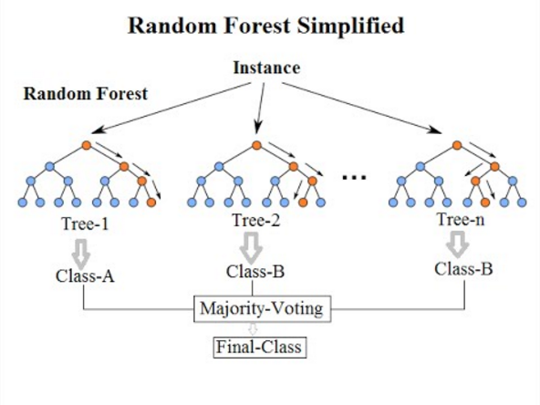
Each individual decision tree within a random forest operates independently and builds its own model for the data set. For any prediction, each tree will independently predict the class, random forest will then decide on the class based on the most predicted (voted) class. There are many ways in which a random forest may assign votes to individual trees. The simplest way is to have one vote for each trees generated. The algorithm could also add weighted votes to each decision tree based on a meta-heuristic.
So in essence, a random forest is a crowd of independent, uncorrelated decision trees that operate as a unit. The large number of trees utilizing many models is expected to outperform any single individual model. The independence of the trees ensure that the features in the data set are modeled is various ways for the same information - thus expanding the solution space in which the algorithm tries to make the prediction.
Having multiple models reduces the error rate as the individual model errors and over-fitting are normalized across all the decision tree models generated. While some trees may be wrong, many other trees will be right, so as a group the trees are able to move in the correct direction when they operate as a unit.
As mentioned above, random forests make use of Decision Trees. It is crucial to to understand how decision trees operate in order to fully grasp the workings of random forests. It is recommended for the reader to go through my previous post on decision trees.
Random Forests generates many classification trees. To classify a new data point, we pass data point down to each of the trees in the forest. Each tree gives an independent classification for that data point ie. the tree “votes” for that class. The forest chooses the classification having the most votes.
Each tree is generated in a random forest as follows:
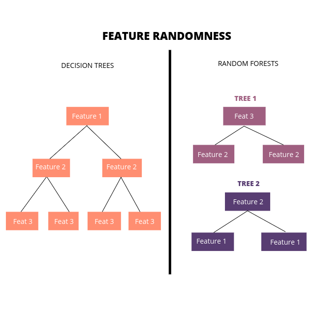
At step 2, unlike decision tree learning, we are not trying to optimize for information gain and get the best feature split. We try to add diversity to our models by utilizing one of the two techniques:
Instead of searching for the most important feature while splitting a node, we search for the best (or random) feature among a random subset of features. This results in a wider diversity that most often result in a better predictions.
For M features in the data set, we take in m random features m < M. At the root nodes of each of the trees generated, we split the data based on this random subset of features.

The Bagging method is more often used in practical implementations. Any model is sensitive to the data it is trained on, so the idea with bagging is to train different trees with different subsets of the data set. In the original paper on random forests with bagging, the ideas was to train decision trees with subset of the data set with replacement ie. all the trees are trained on the same number of features, but with different sections of the data.
In the original paper on random forests, it was shown that the forest error rate depends on two things:
For an optimal classifier, we need low correlation and high strength. Reducing the number of random features (applicable for both Feature Randomness and Bagging) - m - reduces both the correlation and the strength - since lesser number of random features decrease the probability of having highly correlated trees; yet it is unlikely that we will have found a high-accuracy model. Colloquially, increasing it increases both. Somewhere in between is an optimal range of m. This m is the only adjustable parameter to which random forests is somewhat sensitive to.
There are methods to quickly find the optimal value for m like OOB Error.
In practice, Random forests are Swiss army knives of ML algorithms, here are some use cases where they are most useful:
Now that we have understood the algorithm, let’s go ahead and implement it out of box in Python. We can use Python’s all-powerful scikit-learn library to implement Random Forests.
A random forest is a meta estimator that fits a number of decision tree classifiers on various sub-samples of the dataset and uses averaging to improve the predictive accuracy and control over-fitting. The sub-sample size is controlled with the max_samples parameter if bootstrap=True (default), otherwise the whole dataset is used to build each tree.
I’ve used the “Chronic Kidney Diseases” dataset from the UCI ML repository. We will be predicting the presence of chronic kidney disease based on many input parameters. The predict class is binary: “chronic” or “not chronic”.
The dataset will be divided into ‘test’ and ‘training’ samples for cross validation. The training set will be used to ‘teach’ the algorithm about the dataset, ie. to build a model.
In scikit-learn, we can use the sklearn.ensemble.RandomForestClassifier class to perform classification on a dataset. The scikit-learn implementation takes in a variety of input parameters that can be found here. The most interesting of them is the values of n_estimators (the number of trees in the model) and criterion (to specificy the metric for splitting). With the sklearn implementation, you can also provide option for min_samples_split (to specify how may values are needed for a split).
I’ve modified the original data set and have added the header lines. You can find the modified dataset here.
The original dataset has the data description and other related metadata. You can find the original dataset from the UCI ML repo here.
The first thing to do is to read the csv file. To deal with the csv data data, we will use Pandas:
    import pandas as pd
    df = pd.read_csv(r".\data\chronic_kidney_disease.csv") #Reading from the data file
Then non-numerical data elements have to be converted into numerical formats. In this dataset, all the non-numerical elements are of Boolean type. This makes it easy to convert them to numbers. I’ve assigned the numbers ‘4’ and ‘2’ to positive and negative Boolean attributes respectively.
    def mod_data(df):

        df.replace('?', -999999, inplace = True)

        df.replace('yes', 4, inplace = True)

        df.replace('no', 2, inplace = True)

        df.replace('notpresent', 4, inplace = True)

        df.replace('present', 2, inplace = True)

        df.replace('abnormal', 4, inplace = True)

        df.replace('normal', 2, inplace = True)

        df.replace('poor', 4, inplace = True)

        df.replace('good', 2, inplace = True)

        df.replace('ckd', 4, inplace = True)

        df.replace('notckd', 2, inplace = True)
In main.py:
        mod_data(df)

        dataset = df.astype(float).values.tolist()

        #Shuffle the dataset

        random.shuffle(dataset) #import random for this
It is very important to Normalize the dataset - to perform feature scaling. Since the trees are directly sensitive to the magnitude of the parameters. Not normalizing the data prior to distance calculation may reduce the accuracy.
I will be using sci-kit learn’s preprocessing to scale the data.
	from sklearn import preprocessing

        #Normalize the data

        x = df.values #returns a numpy array

        min_max_scaler = preprocessing.MinMaxScaler()

        x_scaled = min_max_scaler.fit_transform(x)

        df = pd.DataFrame(x_scaled) #Replace df with normalized values
Next, we have split the data into test and train - by using test_train_split from scikit-learn.model_selection. In this case, I will be taking 30% of the dataset as the test set:
        #Split data into training and test for cross validation
        X = df.loc[:, df.columns != 24]
        y = df[24]

        # Split dataset into training set and test set
        # 70% training and 30% test
        X_train, X_test, y_train, y_test = train_test_split(X, y, test_size=0.3)
Now that we have the data set ready, we go ahead and fit the data set into our model. For this example, I will run the algorithm with all default features - just to show how well Random Forest works right out of the box.
    clf = RandomForestClassifier(n_estimators=100)
    clf.fit(X_train, y_train)
The test set can now be predicted:
y_pred = clf.predict(X_test)
That’s it.
Now that we have the model fitted, let’s measure the accuracy on the test set. For this, I will use metrics module:
print("Accuracy:", metrics.accuracy_score(y_test, y_pred)*100)
With this, we get:
Accuracy: 98.33333333333333
which is an extremely good value, especially for using the algorithm as a black-box without any parameter estimations. The previously implemented K-Nearest Neighbours only had an accuracy of 88.75
That’s it for now, if you have any comments, please leave then below.