Understanding Genetic Algorithms using an example

What are Genetic Algorithms?

Genetic algorithms are a class of machine learning algorithms which approximate the process of natural selection seen in nature. Genetic algorithms belong to a larger set of Evolutionary algorithms, which take Charles Darwin’s evolution theory as the center piece of inspiration. Genetic algorithms are widely used in solving variety of optimization algorithms in many different domains. Biological processes such as mutation, crossover and selection are heavily relied upon as a source of inspiration in the implementation of generic algorithms.

The main use cases for genetic algorithms are optimization, Classification and Human Comparable Behaviors. Genetic algorithms are essentially a way for of performing biologically inspired optimized trial and error.

In biology, the organisms evolve to suit their environment better, in genetic algorithms, we define the environment (the end result) and we evolve a list of potential solutions until they are converge into an ideal fit to our predefined environment.

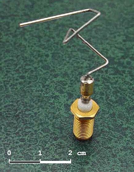
Image courtesy:Wikipedia

The 2006 NASA ST5 spacecraft antenna. This complicated shape was found by an evolutionary computer design program to create the best radiation pattern. It is known as an evolved antenna.

Genetic algorithms are mostly utilized for the following use cases:

• Operations Research
• Biology
• Economics
• AI Design (Like the antenna above)
• Game theory
• Sociology

Genetic algorithms are especially potent in time tabling problems, scheduling problems and generating optimized design, such as designing a network topology.

Prerequisites:

Lets quickly go over and acquaint ourselves with some of the underlying biological concepts that are abstracted in genetic algorithms.

Population and Gene Pool:

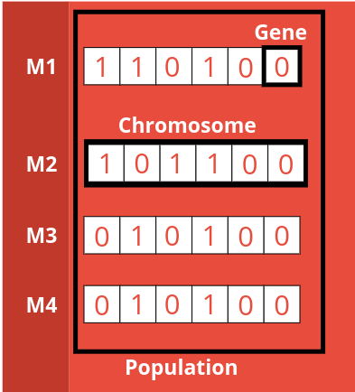
A gene pool is a collection of genetic information in any population. In biology, a gene pool represents the total genetic diversity of population. A gene is the unit information structure, a sequence of genes form a chromosome - which encapsulate all the information about the member - and a population consists of members.

In the application of genetic algorithms, we can abstract the population as a list of potential solutions. In genetic algorithms, each member of a population is a potential solution and would evolve to reach an optimal solution. A gene can be abstracted to a single feature and a chromosome can be abstracted to a single data point with a bunch of features that has all the information to describe it.

Fitness

Fitness involves the ability of populations or species to survive and reproduce in the environment in which they find themselves. The consequence of this survival and reproduction is that organisms contribute genes to the next generation. From the theory of evolution, only the fittest members of the species survive and pass on their genes to the new generation. This way, the new generation are more likely to survive the environment.

In the application of genetic algorithms, we abstract the notion of fitness into a fitness function, which gives a fitness score to each member of the population. The probability that a member will be selected for reproduction is based on its fitness score. In general, the fitness function evaluates how close a member of the population is in relation to the end state.

Cross-Over

Chromosomal crossover, or crossing over, is the exchange of genetic material during reproduction between two members of the population. The new generation created will have genes of both the original members.

In genetic algorithms, we use crossover whilst creating a new generation of population. Only certain members of the population that are more fit than others are chosen for cross over.

Mutation

Biologically, a Mutation occurs when a DNA gene is damaged or changed in such a way as to alter the genetic message carried by that gene. A Mutagen is an agent of substance that can bring about a permanent alteration to the physical composition of a DNA gene such that the genetic message is changed. There are 3 types of biological mutations:

1. Base Substitutions: Involve the swapping of one nucleotide for another during DNA replication ie. swapping one value with another.
2. Deletion: Adding an nucleotide ie. removing a value from a member of the population.
3. Insertions: Adding an extra nucleotide ie. Adding an extra value to a member of the population.

More info on the actual biology can be found here.

In genetic algorithms, the process of mutation inserts a sense of randomness to the population - this enables the algorithm to expand it’s solution set beyond the current values of the population. With mutation, an algorithm can look farther for a solution than the current set of features, since the process of crossover will only re-assemble the existing values.

Mutation also ensures to maintain diversity within the population and prevents premature convergence or over fitting.

Termination

Although in nature evolution keeps going on, we only want to run an algorithm a finite amount of time. For this, genetic algorithms usually have a termination condition. Once this condition is met, the algorithm stops recreating populations and will emit the last created generation as the solution.

Termination conditions usually fall into one of the three:

1. The overall fitness of the population is above a certain, predefined threshold.
2. After many generations, there is no improvement seen in fitness.
3. A predefined absolute number of generations have been created.

How Genetic Algorithms Work:

In genetic algorithms, we generate a random list of population, each member of which can be our potential optimal solution. Using processes like mutation and cross over, we will evolve this population to reach some level “optimality” based on our Selection criteria. Each application of mutation and cross over creates a new generation of population and each new generation of population is more fit and optimal than the previous generation.

Genetic Algorithm Lifecycle:

There are 6 main steps in genetic algorithms:

1. Initial population: Usually randomly generated.
2. Fitness function: A metric to evaluate how fit an abritrary member of population is.
3. Selection: Selecting the most “fit” members of population for the next iteration.
4. Crossover: Reproduction of new generation of members based of the most fit members of the previous generations.
5. Mutation: Adding changes to the new members to maintain diversity and to expand the solution space.
6. Termination: Once a certain condition is met, the algorithm stops creating new generations and emits the solution.

We keep performing steps 2 through 5 until we have reach the optimal composition of the members, at which point we emit the “chromosomes” (The values of the solution).

In case of practical application, before we can create an initial population, first we would have to encode the problem, ie. find a way to represent the problem and the solution space as a sequence of characters.

Solving using genetic algorithm:

I will solve a problem using genetic algorithm to illustrate how the algorithm works.

Problem

Let’s take the example of a simple linear equation:

and solve it using a genetic algorithm.

Encoding

The first step would be encode this problem into a sequence. In this case, we have it pretty simple. We can just encode for the values of a, b and c, the values we are solving for. So, our chromosomes would be a list of 3 values.

Fitness Function

Next, we need to decide on the fitness function. Since we are solving for a linear equation and we have our chromosomes representing the values for a, b and c, we can use the equation itself as the fitness function - by Substituting the values for a, b and c and returning how far it is from the expected result of 15. So we have the Fitness Function:

Termination Condition

We have to decide the termination condition. For our example, the termination would have to happen once the equation is solved - once we find the values for a, b and c that solve the equation ie. when the fitness function returns 0. The termination condition:

Initializing population

Next, we initialize the population - here the size of the population has to be chosen, for the example we will go with a population size of 4. With larger populations, the algorithms explores more of the solution space for a solution - at the cost of computational power.

The population size needs to be chosen meticulously, very large population sizes can slow down computation and in cases of relatively smaller solution spaces can result in many generations exploring the same solutions. Whereas, with a very small population, not enough of the solution space may be explored for an optimal solution.

For this example, we can randomly generate our population - usually in practice one could use a heuristic or an educated guess for initialization.

Initial population:

Solving for the solution

With this initial population and the defined fitness function, we can start applying biological operators to our population and start creating new generations.

First Pass:

Let’s go ahead with the first pass and create a new generation of solutions:

Calculating Fitness:

Selecting members to create the next generations:

The members with the best fitness score [5,2,3] and [2,5,2] have same fitness, we randomly choose one of them - [5,2,3]. We are not choosing the members with the same fitness in order to maintain diversity and to ensure we don’t converge too early. Out of the remaining two, [4,3,3] has better fitness, so that is chosen.

Performing Crossover

We have 2 remaining members from the initial population, these 2 will be used to create the next generation. We will perform cross over to create two new off springs.

Performing Mutation

After crossover, we have the following two: [5,3,3] and [4,2,3], we now mutate these two members to generate two more. We will have 4 members by the end of this process. For this case, I will perform simple insertion (addition of 1) and deletion (subtraction of 1) on random elements in our list.

Which will lead to:

This is the second generation of the population. The above 4 steps are iterated upon until we reach termination, which in this case happens for the 3rd generation where we get the value:

The implementation of the remaining two generations is left as an exercise to the reader.

When should you use Genetic Algorithms?

• When the solution space is less understood or is too big.
• When the solution space is unstructured.
• The presence of multiple conflicting solutions or partial solutions.
• When you need to simulate Human Comparable behaviors(trial and error).
• When the problem to be solved can be approximated to a search in combinatorial space.

In the next article, I will implement Genetic algorithm from scratch in Python.

That’s it for now, if you have any comments, please leave then below.