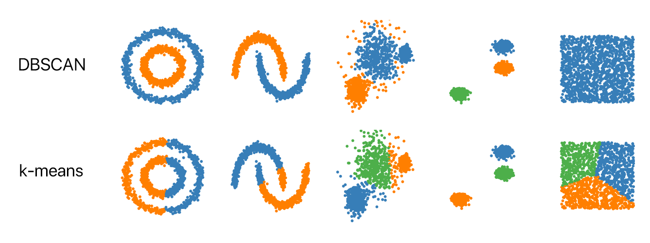
DBSCAN (Density-based spatial clustering of applications with noise) is one of the most popular Machine Learning algorithms for clustering in data mining. One of the prime advantages of DBSCAN is that it’s ability to work with data with significant noise and outliers. Further, DBSCAN does not need to know how many clusters there are in the data set, unlike K-Means clustering.
In this article, I will implement the algorithm from scratch in python and visualize the results on a 2 dimensional data set that, when plotted, forms two concentric circles.
DBSCAN is an unsupervised learning algorithm, ie. it needs no training data, it performs the computation on the actual dataset. This should be apparent from the fact that with DBSCAN, we are just trying to group similar data points into clusters, there is no prediction involved. Unlike previously covered K Means Clustering where we were only concerned with the distance metric between the data points, DBSCAN also looks into the spatial density of data points. Further, DBSCAN can effectively label outliers in the data set based on this density metric - data points which fall in low density areas can be segregated as outliers. This enables the algorithm to be un-distracted by noise.
In my previous blog post, I had explained the theory behind DBSCAN and had implemented the algorithm with Python’s scikit learn. If you are not very familiar with the algorithm or its scikit-learn implementation, do check my previous post.
minPoints, p is a core point and a new cluster is formed.p.The implementation can be divided into the following:
For this implementation, I have chose a simple and contrived 2 dimensional data set that is ideal for the use case of DBSCAN. I have generated the data set using dataset module from sklearn. The data set forms two concentric when plotted on a 2D plane.
The code that I used to generate the data set:
from sklearn import datasets

n_samples = 1500
noisy_circles = datasets.make_circles(n_samples=n_samples, factor=.5, noise=.08)
I have saved a version of this into a csv file which can be found here.
For the implementation, I will use the saved data set of concentric circles instead of generating them for each run.
The first thing to do is to read the csv file. To deal with the csv data data, let’s import Pandas first. Pandas is a powerful library that gives Python R like syntax and functioning.
import pandas as pd
Now, loading the data file:
df = pd.read_csv(r".\data\concentric_circles.csv") #Reading from the data file
Now, lets convert the the data frame into a more generic data structure - a list of floating point numbers:
dataset = df.astype(float).values.tolist()
We can also normalize the data using the StandardScaler from sklearn.preprocessing
from sklearn.preprocessing import StandardScaler

# normalize dataset
X = StandardScaler().fit_transform(dataset)
So far, in main.py:
def main():

  # Reading from the data file
  df = pd.read_csv("./data/concentric_circles.csv")

  dataset = df.astype(float).values.tolist()

  # normalize dataset
  X = StandardScaler().fit_transform(dataset)
Before we move forward, let’s create a class for the algorithm.
  class CustomDBSCAN:
      def __init__(self):
        self.core = -1
        self.border = -2
We have the CustomDBSCAN, that will be our main class for the algorithm. In the constructor, we initialize the arbitrary values for core and border points.
Now, let’s define the functions that go inside the CustomDBSCAN class. For the simplicity of this tutorial, we will not delve into Advanced DBSCAN topics such as the OPTIC algorithm, parameter estimation etc. For our simple implementation, we will only need two functions for the algorithm - fit and neighbour_points. In addition, we will implement a visualize function, to visualize out clusters and outliers.
As their names suggest, the fit function will use the incoming data to model DBSCAN - essentially clustering data based on the provided values of Eps and minPoints. The fit function will use the neighbour_points function to get all the spatially close points to any given point.
First we have the neighbour_points function. The neighbour_points function takes in the pre-processed data set, the index of the current point (pointId) and value of epsilon. The neighbour_points function will return the list of points that are in the Ɛ neighbourhood of any given point.
# Find all neighbour points at epsilon distance
def neighbour_points(self, data, pointId, epsilon):
  pass
Let’s define the fit function. We need the pre-processed data set, the chosen value for Eps and MinPt as params for our function.
# Fit the data into the DBSCAN model
def fit(self, data, Eps, MinPt):
  pass
Next, we have the visualize function. The visualize function takes in the pre-processed data set, the cluster list (returned by the fit function - explained in detail later) and the total number of clusters discovered by DBSCAN . We will be using matplotlib for plotting a scatter plot of the data.
# Visualize the clusters
def visualize(self, data, cluster, numberOfClusters):
  pass
As mentioned above, the neighbour_points function will return all the points in the Ɛ neighbourhood of any arbitrary point in the data set.
For our example, we will be using the Euclidean distance as the distance metric (through there are other options such as the Manhattan Distance, Minkowski Distance ). The Euclidean distance is straight line distance between two data points, that is, the distance between the points if they were represented in an n-dimensional Cartesian plane, more specifically, if they were present in the Euclidean space.
For calculating Euclidean distance, np.linalg.norm function from numpy will be used.
# Find all neighbour points at epsilon distance
def neighbour_points(self, data, pointId, epsilon):
    points = []
    for i in range(len(data)):
        # Euclidian distance
        if np.linalg.norm([a_i - b_i for a_i, b_i in zip(data[i], data[pointId])]) <= epsilon:
            points.append(i)
    return points
The fit function will model the data set to DBSCAN, generating the clusters. The is the core of our implementation.
First, let’s a list that contains which cluster each point belongs to. Initially, as mentioned in the pseudocode, we will mark all the points as outliers. To denote cluster, we can use non-negative integers and we can mark outliers as cluster 0.
    # initialize all points as outliers
    point_label = [0] * len(data)
    point_count = []
Then, we can initialize the empty of list of core and border points:
    # initilize list for core/border points
    core = []
    border = []
We have all the initialized variables ready, we can start with iterating through the data points. I will split the iteration into 3 passes for simplicity. In the first pass, we get all the neighbourhood points for each point. We will utilize the neighbour_points function here:
    # Find the neighbours of each individual point
    for i in range(len(data)):
        point_count.append(self.neighbour_points(data, i, Eps))
In the second pass, we mark the points as core or border/outliers, any point which has more or equal to MinPt number of points in its Ɛ neighbourhood is a core point.
    # Find all the core points, border points and outliers
    for i in range(len(point_count)):
        if (len(point_count[i]) >= MinPt):
            point_label[i] = self.core
            core.append(i)
        else:
            border.append(i)

    for i in border:
        for j in point_count[i]:
            if j in core:
                point_label[i] = self.border
                break
In our final pass, we perform BFS on our data points and assign clusters to each point in our data set. We use the queue data structure to perform BFS.
    # Here we use a queue to find all the neighbourhood points of a core point and find the indirectly reachable points
    # We are essentially performing Breadth First search of all points which are within Epsilon distance for each other
    for i in range(len(point_label)):
        q = queue.Queue()
        if (point_label[i] == self.core):
            point_label[i] = cluster
            for x in point_count[i]:
                if(point_label[x] == self.core):
                    q.put(x)
                    point_label[x] = cluster
                elif(point_label[x] == self.border):
                    point_label[x] = cluster
            while not q.empty():
                neighbors = point_count[q.get()]
                for y in neighbors:
                    if (point_label[y] == self.core):
                        point_label[y] = cluster
                        q.put(y)
                    if (point_label[y] == self.border):
                        point_label[y] = cluster
            cluster += 1  # Move on to the next cluster
This wraps up the fit function. At this stage we have all our points assigned to a cluster (or as an outlier with cluster 0). We can return the list of cluster assignments and the total number of clusters found:
return point_label, cluster
Here’s the entire fit function:
# Fit the data into the DBSCAN model
def fit(self, data, Eps, MinPt):
    # initialize all points as outliers
    point_label = [0] * len(data)
    point_count = []

    # initilize list for core/border points
    core = []
    border = []

    # Find the neighbours of each individual point
    for i in range(len(data)):
        point_count.append(self.neighbour_points(data, i, Eps))

    # Find all the core points, border points and outliers
    for i in range(len(point_count)):
        if (len(point_count[i]) >= MinPt):
            point_label[i] = self.core
            core.append(i)
        else:
            border.append(i)

    for i in border:
        for j in point_count[i]:
            if j in core:
                point_label[i] = self.border
                break

    # Assign points to a cluster

    cluster = 1

    # Here we use a queue to find all the neighbourhood points of a core point and find the
    # indirectly reachable points.
    # We are essentially performing Breadth First search of all points which are within
    # epsilon distance from each other
    for i in range(len(point_label)):
        q = queue.Queue()
        if (point_label[i] == self.core):
            point_label[i] = cluster
            for x in point_count[i]:
                if(point_label[x] == self.core):
                    q.put(x)
                    point_label[x] = cluster
                elif(point_label[x] == self.border):
                    point_label[x] = cluster
            while not q.empty():
                neighbors = point_count[q.get()]
                for y in neighbors:
                    if (point_label[y] == self.core):
                        point_label[y] = cluster
                        q.put(y)
                    if (point_label[y] == self.border):
                        point_label[y] = cluster
            cluster += 1  # Move on to the next cluster

    return point_label, cluster
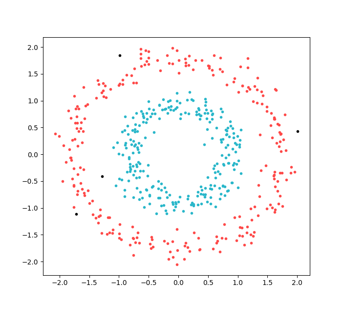
Now that we have our main fit function implemented, let’s quickly write a utility function that visualizes the clusters. We will be using matplotlib.pyplot to plot a scatter plot of all our data points - color coded as per the cluster to which they belong to. In this contrived example, there are clearly two cluster and such as to be shown by the scatter plot.
# Visualize the clusters
def visualize(self, data, cluster, numberOfClusters):
    N = len(data)
    # Define colors, ideally better to have around 7-10 colors defined
    colors = np.array(list(islice(cycle(['#FE4A49', '#2AB7CA']), 3)))

    for i in range(numberOfClusters):
        if (i == 0):
            # Plot all outliers point as black
            color = '#000000'
        else:
            color = colors[i % len(colors)]

        x, y = [], []
        for j in range(N):
            if cluster[j] == i:
                x.append(data[j, 0])
                y.append(data[j, 1])
        plt.scatter(x, y, c=color, alpha=1, marker='.')
    plt.show()
We can completed the implementation of the CustomDBSCAN class. Let’s wrap this implementation by finishing up our main function and looking at the visualized results for the data set. For this exmaple data set, I have found the epsilon and MinPt values to be optimal at 0.25 and 4 respectively.
def main():

    # Reading from the data file
    df = pd.read_csv("./data/concentric_circles.csv")

    dataset = df.astype(float).values.tolist()

    # normalize dataset
    X = StandardScaler().fit_transform(dataset)

    custom_DBSCAN = CustomDBSCAN()
    point_labels, clusters = custom_DBSCAN.fit(X, 0.25, 4)

    print(point_labels, clusters)

    custom_DBSCAN.visualize(X, point_labels, clusters)
The resultant plot:

We have two clear cluster (red and blue), the algorithm splits the concentric circles into separate clusters. We can also see some outliers marked in black.
That’s it for now; if you have any comments, please leave them below.