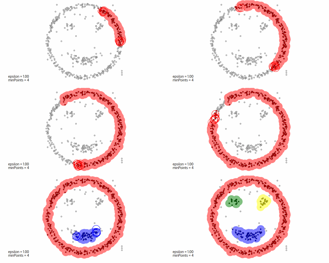
 Image courtesy: Naftali Blog
Density-based Spatial Clustering of Applications with Noise Decision, commonly abbreviated as DBSCAN, is a common data clustering algorithm that is used in data mining and machine learning. DBSCAN is one of the most academically cited methods of clustering data. DBSCAN is especially potent on larger sets of data that have considerable noise; the algorithm works well on odd shaped datasets.
 Image courtesy: Naftali Blog
DBSCAN is an unsupervised learning algorithm, ie. it needs no training data, it performs the computation on the actual dataset. This should be apparent from the fact that with DBSCAN, we are just trying to group similar data points into clusters, there is no prediction involved.
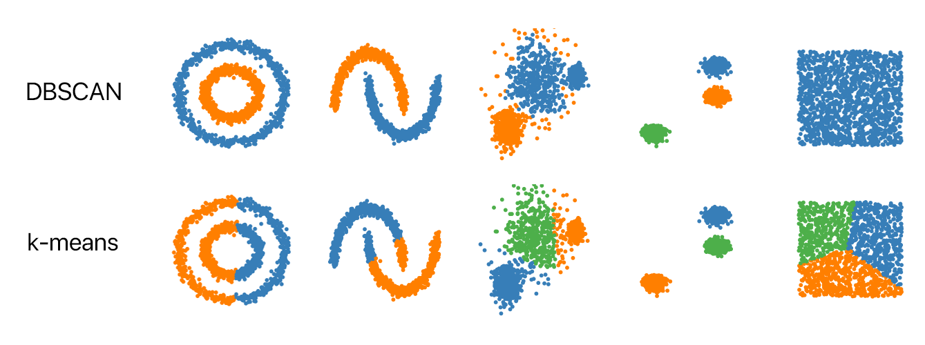
Unlike previously covered K Means Clustering where we were only concerned with the distance metric between the data points, DBSCAN also looks into the spatial density of data points. Further, DBSCAN can effectively label outliers in the dataset based on this density metric - data points which fall in low density areas can be segregated as outliers. This enables the algorithm to be un-distracted by noise.
With DBSCAN, you don’t have to preemptively specify the number of clusters you want in the dataset, unlike k-means. All you need to provide is a value for minimum number of points in a given space and a distance value for what measure of distance is considered “close”.
Before we jump in to the actual workings on the algorithms, we go over a couple concepts that are core to how DBSCAN works.
The Ɛ Neighborhood (Epsilon Neighborhood) is an important concept in the algorithm. Mathematically, it can be defined as:
The set of all points whose distance from a given point is less than some specified number epsilon.
The Ɛ Neighborhood of a point p is a set of all points that are at most some Ɛ (with Ɛ > 0) distance away from it. In a 2D space, such a locus is a circle, with the point p being the center of the circle. In a 3D space, that would be a sphere. Essentially, the Ɛ Neighborhood of a point p is the N Sphere with the point p as the center and the radius being Ɛ.
Smaller the value of Ɛ, the lesser the number of points in the neighborhood of p and vise-versa.
Typically, density is mass/volume; in our case, given a point p we can define:
For example, let’s take the value of Ɛ as 0.5, and take the number of points in the neighborhood as 40, then we have:
This value of density is meaningless in itself, but will play a very significant role in how we cluster the dataset using DBSCAN. In essence, what DBSCAN is actively looking for is dense neighborhoods, with most data points in a relatively small volume.
Now that we have the pre-requisites covered, we can jump right into the algorithm. DBSCAN takes in two parameters:
Ɛ - The radius of the neighborhoods around any arbitrary data point.minPoints - The minimum number of data points we want in a neighborhood to define a cluster.Using these aforementioned data points, DBSCAN classifies each data point into one of three categories:
p, is considered as a core point if the neighborhood at the distance Ɛ has at least minPoints number of data points in it.p, is considered as a border point if the neighborhood at the distance Ɛ has less than minPoints number of data points in it, but p is reachable from at least one of the core points.p, is an outlier if the neighborhood at the distance Ɛ has less than minPoints number of data points in it and p is not reachable from any of the core points.The following image illustrates these three types of categories.
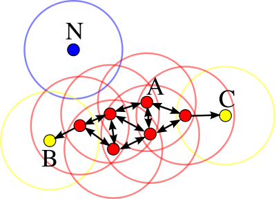 Image courtesy: Wikipedia
In this diagram, minPts = 4. Point A and the other red points are core points, because the area surrounding these points in an ε radius contain at least 4 points (including the point itself). Because they are all reachable from one another, they form a single cluster. Points B and C are not core points, but are reachable from A (via other core points) and thus belong to the cluster as well. Point N is a noise point that is neither a core point nor directly-reachable.
Reach-ability is not a complimentary relation: by definition, only core points can reach non-core points. The opposite is not true, so a non-core point may be reachable, but nothing can be reached from it. You can reach a point q from point p only if p is a core point.
Since Ɛ is fixed - which means the volume is fixed - we essentially have a threshold on the mass. This forces a minimum density requirement on the cluster.
Border points are not core points but are “Density Reachable” by other core points. Here, we have further have two categories of border points:
q is directly density-reachable from object p if p is a core point and q is in the neighborhood of p.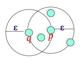
p is indirectly density-reachable from a point q if q is a core point, p is not in the neighborhood of q and p is reachable by another core point, which is reachable by q.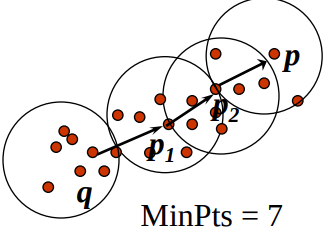
In the next post, I will be implementing the algorithm from scratch in Python, it is recommended to go through that for a more hands-on code based explanation.
Now, let’s list of the steps we’d do to cluster a data set through DBSCAN.
Directly Density Reachable neighbor points to its cluster.Indirect Density Reachable to the origin point). If there is any data point which is labeled as an outlier, change the status and assign it the current cluster - this points are our border points explained above.DBSCAN takes in two parameters and depending on the parameter values might end up with several different clusters for the same dataset. Choosing the right parameter values for Ɛ and minPoints is pivotal to making the algorithm to accurately work to its potential. To choose good parameters one needs to understand how they are used and any knowledge on the dataset will prove to be helpful in making an optimal decision.
Here are some tips whilst choosing the values on the application:
Ɛ- If ε is chosen much too small, a large part of the data will not be clustered; whereas for a too high value of ε, clusters will merge and the majority of objects will be in the same cluster. In general, small values of ε are preferable,[4] and as a rule of thumb only a small fraction of points should be within this distance of each other.
Further, there are algorithms which help you determine the ideal value for Ɛ, something like the K-Nearest Neighbors Graph or Ordering points to identify the clustering structure are routinely used in practice to achieve optimal values for Ɛ
minPoints- As a rule of thumb, a minimum minPoints can be derived from the number of dimensions D in the data set, as minPoints ≥ D + 1. The low value of minPoints = 1 does not make sense, as then every point on its own will already be a cluster. minPoints must be chosen at least 3. However, larger values are usually better for data sets with noise and will yield more significant clusters. As a rule of thumb, minPoints = 2·dim can be used,[7] but it may be necessary to choose larger values for very large data, for noisy data or for data that contains many duplicates.
Further, when implementing this algorithm, one would also have to choose a distance function. The distance between two arbitrary points in an N-dimensional space can take up multiple values depending upon the distance function.
The choice of distance function is tightly coupled to the choice of ε, and has a major impact on the results. In general, it will be necessary to first identify a reasonable measure of similarity for the data set, before the parameter ε can be chosen. There is no estimation for this parameter, but the distance functions needs to be chosen appropriately for the data set. For example, on geographic data, the great-circle distance is often a good choice.
Ɛ and minPoints.Now that we have understood the algorithm, let’s go ahead and implement it out of box in Python. We can use Python’s all-powerful scikit-learn library to implement DBSCAN.
DBSCAN - Density-Based Spatial Clustering of Applications with Noise. Perform DBSCAN clustering from vector array or distance matrix. Finds core samples of high density and expands clusters from them. Good for data which contains clusters of similar density.
In this tutorial, I am going to focus on contrived clustering problems that can be solved using BDSCAN. One could also use scikit-learn library to solve a variety of clustering, density estimation and outlier detection problems. I will be using two toy datasets that make DBSCAN Standout - Two Concentric circles and 2 moons - these are oddly shaped data sets where DBSCAN would outperform other clustering methods like K-Means.
In scikit-learn, we can use the sklearn.cluster.DBSCAN class to perform density based clustering on a dataset. The scikit-learn implementation takes in a variety of input parameters that can be found here. The most interesting of them is the values of eps (which defaults to 0.5) and min_samples (which defaults to 5). With the sklearn implementation, you can also provide option for distance metric (defaults to Euclidean), additional params for the metric, the type of clustering and so on.
As mentioned I will be creating two toy datasets from scikit-learn library. I will be using make_circles and make_moons from the dataset package:
from sklearn import cluster, datasets


np.random.seed(0)

n_samples = 1500
noisy_circles = datasets.make_circles(n_samples=n_samples, factor=.5,
                                      noise=.08)
noisy_moons = datasets.make_moons(n_samples=n_samples, noise=.08)
Now that we have the datasets ready, we go ahead and fit the datasets into our model. For these examples I have chosen the value of eps as 0.2. We will leave the rest of the params to their default value for the sake of simplicity.
eps = 0.2

datasets = [
    noisy_circles,
    noisy_moons,
]
Let’s iterate through the datasets and normalize the dataset. I am going to use the StandardScaler from the library to do so,
for i_dataset, dataset in enumerate(datasets):

    X, y = dataset

    # normalize dataset
    X = StandardScaler().fit_transform(X)
Now we can just initialize the class and fit the data:
    dbscan = cluster.DBSCAN(eps=eps)

    dbscan.fit(X)
Now that we have the model fitted, let’s take in the predicted cluster values and visualize it in matplotlib.
  y_pred = dbscan.labels_.astype(np.int)

  plt.subplot(len(datasets), 1, plot_num)
  if i_dataset == 0:
      plt.title('DBSCAN', size=18)

  colors = np.array(list(islice(cycle(['#FE4A49', '#2AB7CA']), 3)))

  # add black color for outliers (if any)
  colors = np.append(colors, ["#000000"])

  plt.scatter(X[:, 0], X[:, 1], s=10, color=colors[y_pred])

  plt.xlim(-2.5, 2.5)
  plt.ylim(-2.5, 2.5)
  plt.xticks(())
  plt.yticks(())
  plot_num += 1

plt.show()
With this we, have:
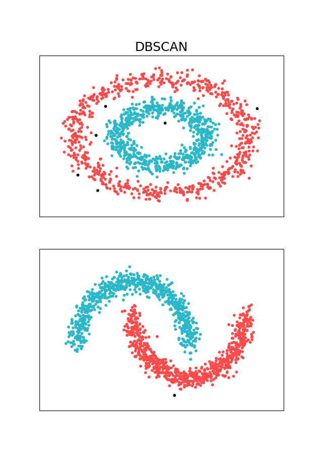
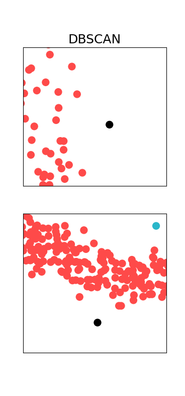
As expected, DBSCAN is able to cluster the dataset in very sensible way. We didn’t have to tell the algorithm how many clusters there might be, it just figured it out. If we zoom in a bit, we can also see the outliers (marked in black):
A comprehensive analysis and visualization of various clustering algorithms on toy datasets can be found in Sklearn’s website. I would recommend for the reader to have a look at that.
That’s it for now, if you have any comments, please leave then below.