Support Vector Machines are perhaps one of the most(if not the most) used classification algorithms. They heralded the downfall of the Neural Networks (It was only in the late 2000s that Neural Nets caught on at the advent of Deep Learning and availability of powerful computers) in the 1990s by classifying images efficiently and more accurately. One of the prime advantages of SVM is that it works very good right out of the box. You can take the classifier in it’s generic form, without any explicit modifications, run it directly on your data and get good results. In addition to their low error rate, support vector machines are computationally inexpensive in contrast to other classification algorithms such as the K Nearest Neighbours.
A Support Vector Machine (SVM) is a discriminative classifier formally defined by a separating hyperplane. In other words, given labeled training data (supervised learning), the algorithm outputs an optimal hyperplane which categorizes new examples.
SVMs are supervised learning algorithms, hence we’ll need to train the algorithm before running it on the actual use case.
Given a set of training examples, each marked as belonging to one or the other of two categories, an SVM training algorithm builds a model that assigns new examples to one category or the other, making it a non-probabilistic binary linear classifier.
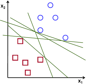
Let us take the example of a linearly seperable set of points on a 2D plane. There is a possibility of many lines or more generally hyperplanes that might cut across datapoints in which that it splits it into the two given classes.

Image courtesy: opencv.org
As can be seen from the above image, there are multiple lines that split the data into the two classes. The question now is, Which is the best line that seperates the two classes? and how do we find it?
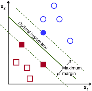
One practical assumption is that, the farther the datapoint is from this separating line, the more confidence we have in our prediction. Naturally, we’d want to make all the points of each class as far as possible from the decision boundary. This can be made sure by having the decision boundary be the farthest from points closest to the decision boundary of each class. Unoptimized decision boundary could result in greater mis-classifications on new data.

Image courtesy: opencv.org
The distance between the closest point and the decision boundary is referred to as margin. In SVMs, all we are really doing is maximizing this margin. The points closest to the separating boundary are referred to as support vectors. Thus, all SVM does is maximize the distance between the separating hyperplane and the support vectors. Simple, yeah?
A hyperplane is a n-1 dimensional Euclidean space that can divide any n dimensional Eucildean space into 2 disconnected parts. A hyperplane can be a point - 0 dimensional, a line - 1 Dimensional, a plane - 2 Dimensional and so on.
Let’s break it down a bit. First, let’s take a line. Now a single point could break that line into two disconnected parts - in this case the said point is the seperating hyperplane. When we take a 2D plane, we can have a line as a separating hyperplane. If we take a 3 dimensional euclidean space, we will need a plane to separate the 3D space into two disconnected parts. Similarly, if we want to split a space with 512 dimensions into two disconnect parts, we will need a 511 Dimensional Euclidean space to do so.
In call the cases, in order to separate an n dimensional Euclidean space, we used a n-1 dimensional Euclidean space. This n-1 Dimensional space is your hyperplane.
d+ : Shortest distance between the decision boundary and the positive support vector
d- : Shortest distance between the decision boundary and the negative support vector
So, d+ + d- = Margin
Equation of the hyperplane:
wT x + b = 0 , where w is the feature vector and b is the bias.
Now, the equation wT x + b = y is used to predict the class (y in the euqation) of any incoming data point. After substituting the param values for w and x, we can decide if the data-point belongs to the class by looking at the sign of y.
To make it easier to understand, let us take the example of a binary set - with classes A and B. w can say that if the value of y for an incoming data point is negative, it belongs to class A. Else if the value of y is positive, we can classify it as B.
We get the equation wT x + b = 0 after a derivation which I am covering in an article on derivation for SVM.
The goal here would be to find a hyperplane such that it splits the dataset into two classes, all while making sure that the margin is maximized. Once we find that optimal separating hyperplane, we can predict the class of new data points.
Now that we have understood the algo, let’s go ahead and implement it out of box in Python. We can use to the all-powerful scikit-learn library to implement SVM.
The support vector machines in scikit-learn support both dense (numpy.ndarray and convertible to that by numpy.asarray) and sparse (any scipy.sparse) sample vectors as input.
In this tutorial, I am going to focus on classification problems that can be solved using SVMs. One could also use scikit-learn library to solve a variety of regression, density estimation and outlier detection.
In scikit-learn, we can use the sklearn.svm.SVC, sklearn.svm.NuSVC and sklearn.svm.LinearSVC classes to perform multi-class classification on a dataset. SVC and NuSVC are based on libsvm and LinearSVC is based on liblinear.
SVC, NuSVC and LinearSVC take as input two arrays: an array X of size [n_samples, n_features] holding the training samples, and an array y of class labels (strings or integers), size [n_samples]
Let’s try out a very simple example of SVC, with linearly separable binary set:
from sklearn import svm

data = [[1,1], [6,6]]
y = [1,6]
clf = svm.SVC()
clf.fit(data, y)
# Print out the support vectors
print(clf.support_vectors_)
# Let us make a prediction
print(clf.predict([[5.,5.]]))
Let’s do the same for multi-class classification:
from sklearn import svm

data = [[1,1], [2,2], [3,3], [4,4]]
y = [1,2,3,4]
# For multi class calssification
clf = svm.SVC(decision_function_shape = 'ovr')
clf.fit(data, y)
# Print out the support vectors
print(clf.support_vectors_)
# Let us make some predictions
print(clf.predict([[5.,5.]]))
print(clf.predict([[1.,2.]]))
Now, let us work on some real data. I have with me a dataset with 2 parameters and 2 classes. You can find thedataset here.
The first thing to do is to read the csv file. To deal with the csv data data, let’s import Pandas first. Pandas is a powerful library that gives Python R like syntax and functioning. After that we just read the file and seperate out feature and the class columns into X and y. We will be feeding the X and y into our SVM classifier class’ fit function. Usually the first thing to do whilst working on SVMs is to convert the non-numerical data elements into numerical formats. In our dataset, however, we only have numerical values, so we’re good to go as is.
import pandas as pd

def main():
	df = pd.read_csv(r"fourclass.tsv", sep = "\t")
	dataset = df.astype(float).values.tolist()
	print(df.head()) #Sample of the dataset

	# Split into feature and class arrays
	X = np.array(df.drop(['class'], 1))
	y = np.array(df['class'])
The predict class is binary: “1” or “0”. The dataset will be divided into ‘test’ and ‘training’ samples for cross validation. The training set will be used to ‘teach’ the algorithm about the dataset, ie. to build a model. The test set will be used for evaluation of the results.
Let us split the data into test and train. In this case, I will be taking 20% of the dataset as the test set. We can can use sklearn’s cross_validation method to get this done:
from sklearn import cross_validation

def main()
	....

	X_train, X_test, y_train, y_test = cross_validation.train_test_split(X, y, test_size = 0.2)
Now, let’s fit the data into our classifier
clf = svm.NuSVC(decision_function_shape = 'ovo')
clf.fit(X_train, y_train)
Yep, it’s that simple(to start with).
The decision_function_shape by default is ovr - One vs rest type multi-classifier. The other option is ovo - one vs one classifier.
Now, let’s find the accuracy
accuracy = clf.score(X_test, y_test)
print(accuracy)

>> 0.9
Not bad. We can now make a prediction using the clf.predict() method.
example_measure = [[11,1]]
prediction = clf.predict(example_measure)
print(prediction)

>> [1]
In order to effectively visualize the SVM’s output, I will gonna go ahead and use mlxtend. Mlextend has has a pretty effective plotting function for visualizing SVMs through decision regions. It actually matplotlib under the hood, so we need to import and plot using matplotlib when using mlxtend.
Let’s import!
from mlxtend.plotting import plot_decision_regions
import matplotlib.pyplot as plt
Now, once we have fit our data, we can use the plot_decision_regions method from the mlxtend library.
plot_decision_regions(X=X, y=y, clf=clf, legend=2)
plt.xlabel("x", size=5)
plt.ylabel("y", size=5)
plt.title('SVM Decision Region Boundary', size=6)
plt.show()
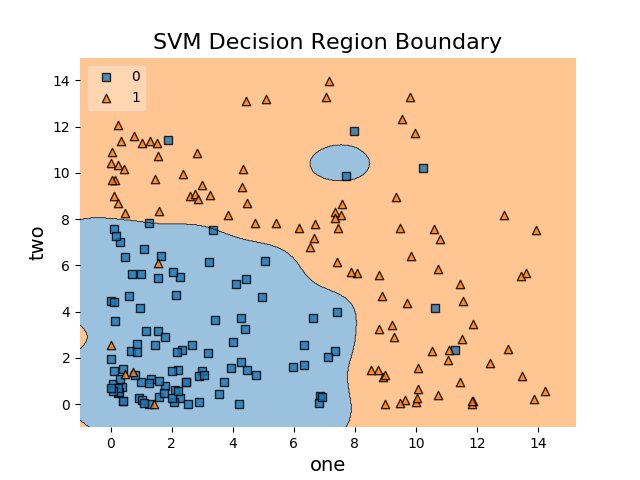
Here’s what we get

As we can see, the decision boundaries look alright and it can be observed that the margin is perhaps as large as it can be.
Here’s the final code:
from sklearn import cross_validation, svm
import pandas as pd
import numpy as np
from mlxtend.plotting import plot_decision_regions
import matplotlib.pyplot as plt

def main():
	df = pd.read_csv(r"data.tsv", sep = "\t")
	dataset = df.astype(float).values.tolist()
	print(df.head())

	X = np.array(df.drop(['class'], 1))
	y = np.array(df['class'])

	X_train, X_test, y_train, y_test = cross_validation.train_test_split(X, y, test_size = 0.2)

	clf = svm.NuSVC(decision_function_shape = 'ovo')
	clf.fit(X_train, y_train)

	accuracy = clf.score(X_test, y_test)


	print(accuracy)

	plot_decision_regions(X=X,
                      y=y,
                      clf=clf,
                      legend=2)

	plt.xlabel("one", size=14)
	plt.ylabel("two", size=14)
	plt.title('SVM Decision Region Boundary', size=16)
	plt.show()
	example_measure = [[11,1]]
	prediction = clf.predict(example_measure)
	print(prediction)

if __name__ == "__main__":
	main()
That’s it for now, if you have any comments, please leave them below.