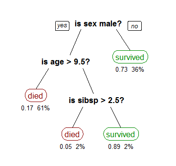
Decision tree learning is one of the most commonly known machine learning algorithms out there. One of the advantages of decision trees are that there are quite staright forward, easily understandable by humans. Decision trees provide a way to approximate discrete valued functions and are robust to noisy data. Decision trees can be represented using the typical Tree Data Structure.
Decision tree learning uses a decision tree (as a predictive model) to go from observations about an item (represented in the branches) to conclusions about the item’s target value (represented in the leaves). It is one of the predictive modelling approaches used in statistics, data mining and machine learning.
In decision tree learning, a decision tree - now known by the umbrella term CART (Classification and Regression Tree) - can be used to visually and explicitly represent decisions and decision making. Though, it is common to use a tree-like model for decisions, learned trees can also be represented as sets of if-else-then rules.
Though decision trees can be utilized for both classification and regression, it’s primarily used for classification.
Decision trees perform classification after sorting the instances in a top-down approach - from the root to the leaf. Each non-leaf node splits the set of instances based on a test of an attribute. Each branch emanting from a node corresponds to one of the possible values of the said attribute in the node. The leaves of the decision tree specifies the label or the class in which a given instance belongs to.
Here’s an example of a classification tree (Titanic Dataset):

Image courtesy: Wikipedia
The above model uses three attributes namely : Gender, age and number of spouses/children. As can be seen from the example, the internal nodes have an attribute test associated with them. This test splits the data set based on the value of the said attribute of the incoming instance. The branches correspond to the values of the attribute in question. At the end, the leaf node represent the class of the instance - in this case the fate of the titanic passengers.
Decision Trees represent a disjunction of conjunctions of constraints on attributes values of instances.
That is, Decision Trees represent a bunch of AND ‘statements’ chained by OR statements. For example, let’s look at the titanic example above. The given tree can be represented by a disjunction of conjuctions as: ( female ) OR ( male AND less than 9.5 years of age AND more than 2.5 siblings)
Before we start classifying, we first need to build the tree from the available dataset.
Most algorithms that have been developed for learning decision trees are variations of the core algorithm that employs a top down, greedy search through the possible space of decision trees.
In this article, I will be focussing on the Iterative Dichotomiser 3, commonly know as the ID3 algorithm. Variants/Extensions of the ID3 algorithm, such as C4.5, are very much in practical use today.
The ID3 algorithm builds the tree top-down, starting from the root by meticulously choosing which attribute that will be tested at each given node. Each attribute is evaluated through statistical means as to see which attribute splits the dataset the best. The best attribute is made the root, with it’s attribute values branching out. The process continues with the rest of the attributes. Once an attribute is selected, it is not possible to backtrack.
Entropy is a measure of unpredictability of the state, or equivalently, of its average information content.
Entropy is a statistical metric that measures the impurity. Given a collection of S, which contains two classes: Positive and Negative, of some arbitrary target concept, entropy with respect to this boolean classification is:
Entropy(S) = E(S) = -ppositivelog2 p positive - pnegativelog2 p negative
Where ppositive is the proportion (probability) of positive examples in S and pnegative is the proportion of negative examples in S. Entropy is 1 if the collection S contains equal number of examples from both classes, Entropy is 0 if all the examples in S contain the same example.
The entropy values vs the probabilities for a collection S follows a parabolic curve:
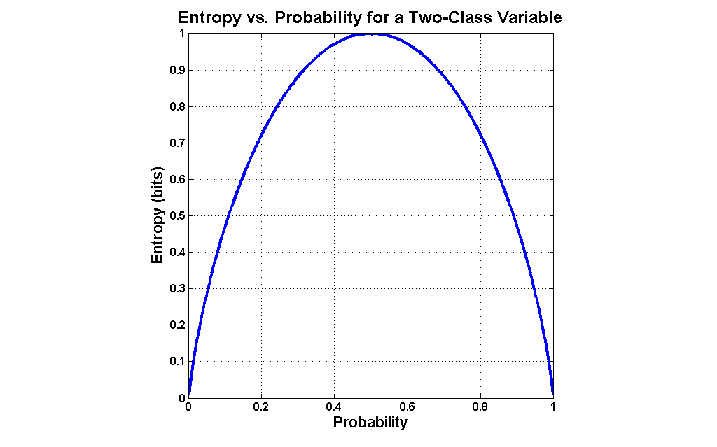
Image courtesy: MATLAB data science
One interpretation of entropy is that, entropy specifies the minimum number of bits required to encode the classification of any member of a collection S.
In general terms, when the classes of the target function may not always be boolean, entropy is defined as

Now that we know what entropy is, let’s look at an attribute that is more attached to the building of the decision tree - Information Gain. Information gain is a metric that measures the expected reduction in the impurity of the collection S, caused by splitting the data according to any given attribute.
The information gain IG(S,A) of an attribute A, from the collection S, can be defined as
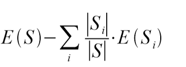
Image courtesy: Abhyast
where i spans through the entire set of all possible values for attribute A, and S i is the portion of S for which attribute A has the value i. The first term is the entropy of the entire collection S. One way to think about IG is that, the value of IG is the number of bits saved when encoding a target value of an arbitrary member of the collection.
Whilst building the decision tree, the information gain metric is used by the ID3 algorithm to select the best attribute - the attribute the provides the “best split” - at each level.
Let’s take the example of a dataset. This dataset assesses the risk of tumour in a patient. We will be generating a decision tree using the ID3 algorithm.
| HEADACHE | DIZZYNESS | BLOOD PRESSURE | RISK |
| YES | NO | HIGH | YES |
| YES | YES | HIGH | YES |
| NO | NO | NORMAL | NO |
| YES | YES | NORMAL | YES |
| YES | NO | NORMAL | NO |
| NO | YES | NORMAL | YES |
First, let’s find the entropy of the entire collection:
E(S) = -pyes log2 pyes - pno log2 pno
From the dataset: pyes = 4/6 and pno = 2/6
So, E(S) = - { (4/6) log2(4/6) } - { (2/6) log2(2/6) }
This gives us E(S) = 0.9182
Now, the information gain, let’s consider the attribute HEADACHE. This attribute has two values YES and NO. Now, the proportion of YES in the attribute: 4/6 and the proportion of NO in the attribute: 2/6
Hence, the split:
SYES - [3+, 1-] ( 3 positive and 1 negative classification when HEADACHE has the value YES)
SNO - [0+, 2-] ( 2 negative classifications when HEADACHE has the value NO)
Therefore,
IG(S, HEADACHE) = E(S) - (4/6) * E(SYES) - (2/6) * E(SNO).
After Calculation: IG(S, HEADACHE) = 0.37734.
Similarly, IG(S, DIZZYNESS) = 0.4590 and IG(S, BP) = 0.5848
After we have calculated the information for these attributes, we choose the attribute with the highest information gain as the splitting attribute for the node. This process goes on top-down until we are left we just leaves - the classification. From above, it is clear that the attribute BLOOD PRESSURE will be our attribute of choice at the root node.
Splitting at the root node using BLOOD PRESSURE gives us the following tree:
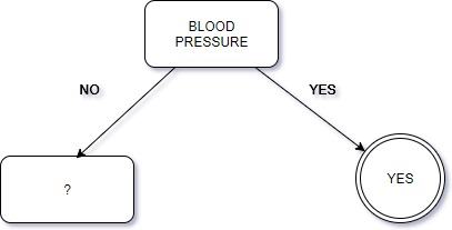
If the value of BLOOD PRESSURE is YES then we directly arrive at the class being YES. If the value is no, we need to split the dataset again and the child node. As said, this is a top-down approach.
Now, let’s move to choosing the next splitting attribute. The process is essentially the same, except we now consider the rows where the value of the BLOOD PRESSURE attribute is NO.
pyes = 2/4 and pno = 2/4
So, E(S) = - { (2/4) log2(2/4) } - { (2/4) log2(2/4) }
This gives us E(S) = 1.0
After calculations similar as above, we find IG(HEADACHE) = 0 and IG(DIZZYNESS) = 1. We now choose the DIZZYNESS attribute as the splitting attribute. This gives us the final decision tree, using which we can predict the classification. Notice that we don’t have to use the HEADACHE attribute since, from the given data, we can make predictions based upon the other two attributes.
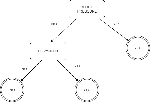
The ID3 algorithm usually prefers shorter, wider trees over the taller ones. The trees which has a high information gain are placed closer to the root.
As the data that is fed becomes larger, the decision tree tends to become longer. In such cases, noise and corrupt/incorrect data can have a detrimental impact on the decision tree. This results in the decision tree overfitting the dataset, that is decision tree performs satisfactory for the training data, but fails to produce an appropriate approximation of the target concept when it encounters actual data. Overfitting can also occur when insufficent data is provided to build the decision tree (like perhaps, our previous with only 6 rows.)
In order overcome the overfitting scenario, one of the following two things must be done. Either the decision tree should stop growing before it overfits the data or an overfitting tree should be pruned to reduce the error.
That’s it for now, if you have any comments, please leave then below.