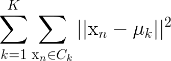
K Means Clustering is one of the most popular Machine Learning algorithms for cluster analysis in data mining. K-means clustering aims to partition n observations into k clusters in which each observation belongs to the cluster with the nearest mean, serving as a prototype of the cluster.
K Means algorithm is an unsupervised learning algorithm, ie. it needs no training data, it performs the computation on the actual dataset. This should be apparent from the fact that in K Means, we are just trying to group similar data points into clusters, there is no prediction involved.
The K Means algorithm is easy to understand and to implement. It works well in a large number of cases and is a powerful tool to have in the closet.
The algorithm has a loose relationship to the k-nearest neighbor classifier, a popular machine learning technique for classification.
One can apply the 1-nearest neighbor classifier on the cluster centers obtained by k-means to classify new data into the existing clusters.
The K Means algorithm is iterative based, it repeatedly calculates the cluster centroids, refining the values until they do not change much.
The k-means algorithm takes a dataset of ‘n’ points as input, together with an integer parameter ‘k’ specifying how many clusters to create(supplied by the programmer). The output is a set of ‘k’ cluster centroids and a labeling of the dataset that maps each of the data points to a unique cluster.
The math:

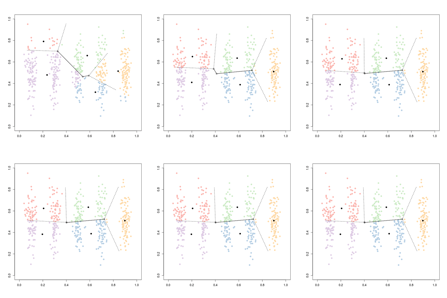
Image courtesy: DSlab
In the beginning, the algorithm chooses k centroids in the dataset. Then it calculates the distance of each point to each centroid. Each centroid represents a cluster and the points closest to the centroid are assigned to the cluster. At the end of the first iteration, the centroid values are recalculated, usually taking the arithmetic mean of all points in the cluster.
After the new values of centroid are found, the algorithm performs the same set of steps over and over again until the differences between old centroids and the new centroids are negligible.
K Means in action

I’ve used the IPL stats dataset that I compiled from inline sources. We will be clustering the cricket players based on their batting and bowling performance. I am using a normalized dataset and hence, I will not be normalizing it in my code.
I shall visualize the algorithm using the mathplotlib module for python.
The implementation can be divided into the following:
Before we move forward, let’s create a class for the algorithm.
class K_Means:

	def __init__(self, k =3, tolerance = 0.0001, max_iterations = 500):
		self.k = k
		self.tolerance = tolerance
		self.max_iterations = max_iterations
In the constructor, I have set the default number of cluster, ie. the value of k as 3. So, by default the implementation will form 3 clusters out of the dataset. I’ve set teh tolerance value as 0.0001. When the difference between the old and new centroids is less than the tolerance value, we stop the iterations. The final argument is the max_iterations which specifies the maximum number of times the algorithm can iterate trying to optimize the centroid values, the default value is set to 500 iterations. So, by default, teh algorithm stops when the difference between the old and the new centroids is less than 0.0001x or when the number of iterations has crossed 500.
I’m using the normalized data set and have added the header lines. You can find the dataset here.
The first thing to do is to read the csv file. To deal with the csv data data, let’s import Pandas first. Pandas is a powerful library that gives Python R like syntax and functioning.
import pandas as pd
Now, loading the data file:
df = pd.read_csv(r".\data\ipl_bowlers_norm.csv")
In main.py:
df = df[['one', 'two']]
dataset = df.astype(float).values.tolist()

X = df.values #returns a numpy array
The k-means algorithm, like the k-NN algorithm, relies heavy on the idea of distance between the data points and the centroid. This distance is computed is using the distance metric. Now, the decision regarding the decision measure is very, very imperative in k-Means. A given incoming point can be predicted by the algorithm to belong one cluster or many depending on the distance metric used. From the previous sentence, it should be apparent that different distance measures may result in different answers.
There is no sure-shot way of choosing a distance metric, the results mainly depend on the dataset itself. The only way of surely knowing the right distance metric is to apply different distance measures to the same dataset and choose the one which is most accurate.
In this case, I will be using the Euclidean distance as the distance metric (through there are other options such as the Manhattan Distance, Minkowski Distance ). The Euclidean distance is straight line distance between two data points, that is, the distance between the points if they were represented in an n-dimensional Cartesian plane, more specifically, if they were present in the Euclidean space.
From Wikipedia:
In Cartesian coordinates, if p = (p1, p2,…, pn) and q = (q1, q2,…, qn) are two points in Euclidean n-space, then the distance (d) from p to q , or from q to p is given by:
import math

def Euclidean_distance(feat_one, feat_two):

    squared_distance = 0

    #Assuming correct input to the function where the lengths of two features are the same

    for i in range(len(feat_one)):

            squared_distance += (feat_one[i] – feat_two[i])**2

    ed = sqrt(squared_distances)

    return ed;
The above code can be extended to n number of features. In this example, however, I will rely on Python’s numpy library’s function: numpy.linalg.norm
After figuring out the distances between the points, we will use the distances to find which cluster amongst the k clusters a given data point belongs to.
First, let’s initialize the centroids randomly:
#initialize the centroids, the first 'k' elements in the dataset will be our initial centroids
for i in range(self.k):
	self.centroids[i] = data[i]
Now, let’s enter the main loop.
for i in range(self.max_iterations):
		self.classes = {}
		for i in range(self.k):
			self.classes[i] = []

		#find the distance between the point and cluster; choose the nearest centroid
		for features in data:
			distances = [np.linalg.norm(features - self.centroids[centroid]) for centroid in self.centroids]
			classification = distances.index(min(distances))
			self.classes[classification].append(features)
The main loop executes max_iterations number of times at most. We are defining the each cluster in the classes list. Then we iterate through the features in data and find the distance between the features of the data point and the features of the centroid. After finding the cluster nearest to the datapoint, we append the cluster list within classes with the data point’s feature vector.
Now, let’s re-calculate the cluster centroids.
previous = dict(self.centroids)

#average the cluster datapoints to re-calculate the centroids
for classification in self.classes:
	self.centroids[classification] = np.average(self.classes[classification], axis = 0)
The dictionary previous stores the value of centroids that the previous iteration returned, we performed the clustering in this iteration based on these centroids. Then we iterate though the classes list and find the average of all the datapoints in the given cluster. This is, perhaps, the machine learning part of k-means. The algorithm recomputes the centroids as long as it’s optimal(or if there have been far too many interations in attempting to do so).
Time to see if our algorithm has reached the optimal values of centroids. For this, let’s have a flag isOptimal.
isOptimal = True
Let’s iterate though the new centroids and compare it with the older centroid values and see if it’s converged.
for centroid in self.centroids:

	original_centroid = previous[centroid]
	curr = self.centroids[centroid]

	if np.sum((curr - original_centroid)/original_centroid * 100.0) > self.tolerance:
		isOptimal = False

	#break out of the main loop if the results are optimal, ie. the centroids don't change their positions much(more than our tolerance)

if isOptimal:
		break
We find the situation to be optimal if the percentage change in the centroid values is lower than our accepted value of tolerance. We break out of the main loop if we find that the algorithm has reached the optimal stage, ie. the changes in the values of centroids, if the algorithm continued to execute, is negligible.
Now that we are done with clustering, let us visualize the datasets to see where these clusters stand at. I will be using python matplotlib module to visualize the dataset and then color the different clusters for visual identification.
In main:
km = K_Means(3)
km.fit(X)

# Plotting starts here, the colors
colors = 10*["r", "g", "c", "b", "k"]
Lets mark our centroids with an x.
for centroid in km.centroids:
	plt.scatter(km.centroids[centroid][0], km.centroids[centroid][1], s = 130, marker = "x")
Now, let’s go ahead and plot the datapoints and color them based on their cluster.
for classification in km.classes:
	color = colors[classification]
	for features in km.classes[classification]:
		plt.scatter(features[0], features[1], color = color,s = 30)
Show the plot:
plt.show()
Output:
Here we have our scatter plot with clustering done on it using K Means clustering algorithm. The three clusters can be thought of as Batsmen (Red), Bowlers(Green) and Allrounders(Blue).
That’s it for now; if you have any comments, please leave them below.