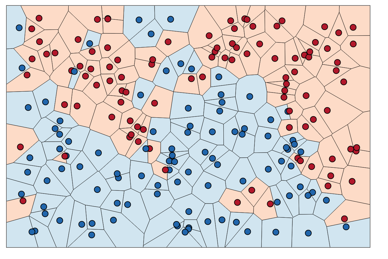
Implementing K Nearest Neighbours from Scratch - in Python

K Nearest Neighbours is one of the most commonly implemented Machine Learning classification algorithms. The kNN is more widely used in classification problems than for regression problems, although it can be applied for both classification and regression problems.

The kNN algorithm is easy to understand and to implement. It works well in a large number of cases and is a powerful tool to have in the closet.

The k-NN algorithm derives much of its power from the fact that it’s non-parametric; this means that the algorithm has no prior bias or a functional form. It does not make any assumptions about the dataset in hand.

How k-NN works:

k-NN algorithm uses the entire training dataset as its model. For a new prediction to come out of k-NN, the algorithm will scour the entire training data to find ‘k’ points nearest to the incoming data. Then, depending on the class of these ‘k’ points, the probable class of the incoming data is predicted.

The computation only happens on the arrival of new data. Each time a new data-point is fed into k-NN, it will again search through the entire dataset to find those ‘k’ points. The algorithm does not build any model until the time a classification-based prediction is required. This technique of performing all the computation whilst the classification(ie. in the end) is referred to as lazy learning or instance based-learning.

Predict the presence of Chronic Kidney disease:

I’ve used the “Chronic Kidney Diseases” dataset from the UCI ML repository. We will be predicting the presence of chronic kidney disease based on many input parameters. The predict class is binary: “chronic” or “not chronic”.

The dataset will be divided into ‘test’ and ‘training’ samples for cross validation. The training set will be used to ‘teach’ the algorithm about the dataset, ie. to build a model; which, in the case of k-NN algorithm happens during active runtime during prediction. The test set will be used for evaluation of the results.

Implementing k-NN:

Setting up the class:

class CustomKNN:

    #constructor

    def __init__(self):

            self.accurate_predictions = 0

            self.total_predictions = 0

            self.accuracy = 0.0

Handling Data:

I’ve modified the original data set and have added the header lines. You can find the modified dataset here.

The original dataset has the data description and other related metadata. You can find the original dataset from the UCI ML repo here.

The first thing to do is to read the csv file. To deal with the csv data data, let’s import Pandas first. Pandas is a powerful library that gives Python R like syntax and functioning.

import pandas as pd

df = pd.read_csv(r".\data\chronic_kidney_disease.csv") #Reading from the data file

The first thing is to convert the non-numerical data elements into numerical formats. In this dataset, all the non-numerical elements are of Boolean type. This makes it easy to convert them to numbers. I’ve assigned the numbers ‘4’ and ‘2’ to positive and negative Boolean attributes respectively.

def mod_data(df):

    df.replace('?', -999999, inplace = True)

    df.replace('yes', 4, inplace = True)

    df.replace('no', 2, inplace = True)

    df.replace('notpresent', 4, inplace = True)

    df.replace('present', 2, inplace = True)

    df.replace('abnormal', 4, inplace = True)

    df.replace('normal', 2, inplace = True)

    df.replace('poor', 4, inplace = True)

    df.replace('good', 2, inplace = True)

    df.replace('ckd', 4, inplace = True)

    df.replace('notckd', 2, inplace = True)

    mod_data(df)

    dataset = df.astype(float).values.tolist()

    #Shuffle the dataset

    random.shuffle(dataset) #import random for this

Next, we have split the data into test and train. In this case, I will be taking 25% of the dataset as the test set:

    #25% of the available data will be used for testing

    test_size = 0.25

    #The keys of the dict are the classes that the data is classified into

    training_set = {2: [], 4:[]}

    test_set = {2: [], 4:[]}

Now, split the data into test and training; insert them into test and training dictionaries:

    #Split data into training and test for cross validation

    training_data = dataset[:-int(test_size \* len(dataset))]

    test_data = dataset[-int(test_size \* len(dataset)):]

    #Insert data into the training set

    for record in training_data:
			#Append the list in the dict will all the elements of the record except the class
            training_set[record[-1]].append(record[:-1])

    #Insert data into the test set

    for record in test_data:
			# Append the list in the dict will all the elements of the record except the class
            test_set[record[-1]].append(record[:-1])

Distance Calculation:

Normalizing Dataset:

Before calculating distance, it is very important to Normalize the dataset - to perform feature scaling. Since the distance measure is directly dependent on the magnitude of the parameters, the features with higher average values will get more preference whilst decision making; for example, in the dataset in our case, the feature ‘age’ might get more preference since its values are higher than that of other features. Not normalizing the data prior to distance calculation may reduce the accuracy.

from sklearn import preprocessing

    #Normalize the data

    x = df.values #returns a numpy array

    min_max_scaler = preprocessing.MinMaxScaler()

    x_scaled = min_max_scaler.fit_transform(x)

    df = pd.DataFrame(x_scaled) #Replace df with normalized values

Distance Metric:

The k-NN algorithm relies heavy on the idea of similarity of data points. This similarity is computed is using the distance metric. Now, the decision regarding the decision measure is very, very imperative in k-NN. A given incoming point can be predicted by the algorithm to belong one class or many depending on the distance metric used. From the previous sentence, it should be apparent that different distance measures may result in different answers.

There is no sure-shot way of choosing a distance metric, the results mainly depend on the dataset itself. The only way of surely knowing the right distance metric is to apply different distance measures to the same dataset and choose the one which is most accurate.

In this case, I will be using the Euclidean distance as the distance metric (through there are other options such as the Manhattan Distance, Minkowski Distance ). The Euclidean distance is straight line distance between two data points, that is, the distance between the points if they were represented in an n-dimensional Cartesian plane, more specifically, if they were present in the Euclidean space.

Implementing Euclidean distance for two features in python:

import math

def Euclidean_distance(feat_one, feat_two):

    squared_distance = 0

    #Assuming correct input to the function where the lengths of two features are the same

    for i in range(len(feat_one)):

            squared_distance += (feat_one[i] – feat_two[i])**2

    ed = sqrt(squared_distances)

    return ed;

The above code can be extended to n number of features. In this example, however, I will rely on Python’s numpy library’s function: numpy.linalg.norm

Prediction:

After figuring out the distances between the points, we will use the distances to find the ‘k’ nearest neighbours of the given point and then, based on the classes of these ‘neighbours’, make the prediction on the class of the incoming data.

This is quite straight-forward: First calculate the distance between the incoming point and all the points in the training set. Then select a subset of size k from those points and find the probability of the incoming point being in each class. The class with the most probability will be selected as the predicted class.

We get to choose the value ‘k’. There are many rules of thumb to do this, but most often the value of ‘k’ is chosen after trail and error. In this case, I am setting the default value of k to 3.

def predict(self, training_data, to_predict, k = 3):

            if len(training_data) >= k:

                    print("K cannot be smaller than the total voting groups(ie. number of training data points)")

                    return

            distributions = []

            for group in training_data:

                    for features in training_data[group]:

                            euclidean_distance = np.linalg.norm(np.array(features)- np.array(to_predict))

                            distributions.append([euclidean_distance, group])

                    results = [i[1] for i in sorted(distributions)[:k]]

                    result = Counter(results).most_common(1)[0][0]

                    confidence = Counter(results).most_common(1)[0][1]/k

            return result, confidence

Testing/Evaluation :

Now that we have finished up the algorithm, it’s time to test how well it performs. Since, for this dataset, k-NN is a bindary classifier, I will be using classification accuracy to evaluate the algorithm.

def test(self, test_set, training_set):
	for group in test_set:
		for data in test_set[group]:

			#Making the predictions

			predicted_class,confidence = self.predict(training_set, data, k =3)

			if predicted_class == group: #Got it right
				self.accurate_predictions += 1
			else:
				print("Wrong classification with confidence " + str(confidence * 100) + " and class " + str(predicted_class))

			self.total_predictions += 1

	self.accuracy = 100*(self.accurate_predictions/self.total_predictions)
	print("	nAcurracy :", str(self.accuracy) + "%")

Along with the classification accuracy, above function will also print out the wrongly classified elements with the probablities.

>>>Accuracy: 88.75%

Comparing accuracy of Custom k-NN with sci-kit k-NN:

Now, let’s compare our implmentation with the sci-kit learn implementation. This is just for demonstration purposes only. If I was using k-NN algorithm in a production environment, I would definitely use the library function and so should you.

from sklearn import preprocessing, cross_validation, neighbors
import pandas as pd
import numpy as np


def mod_data(df):

	df.replace('?', -999999, inplace = True)

	df.replace('yes', 4, inplace = True)
	df.replace('no', 2, inplace = True)

	df.replace('notpresent', 4, inplace = True)
	df.replace('present', 2, inplace = True)

	df.replace('abnormal', 4, inplace = True)
	df.replace('normal', 2, inplace = True)

	df.replace('poor', 4, inplace = True)
	df.replace('good', 2, inplace = True)

	df.replace('ckd', 4, inplace = True)
	df.replace('notckd', 2, inplace = True)



df = pd.read_csv(r".\data\chronic_kidney_disease.csv") #Reading from the data file
mod_data(df)

X = np.array(df.drop(['class'], 1))
y = np.array(df['class'])

#Use 25% of the data as test
X_train, X_test, y_train, y_test = cross_validation.train_test_split(X, y, test_size = 0.25)

clf = neighbors.KNeighborsClassifier()
clf.fit(X_train, y_train)

accuracy = clf.score(X_test, y_test)

print("Accuracy: " + str(accuracy*100) + "%")

>>>Accuracy: 86.75%

However, in most runs, the accuracy hovered around the value of 81.25%. I was quite surprised at the result myself. I am not fully sure as to why the custom implementation slightly out-performed the sci-kit learn implementation. This probably has something to do with the fact that I have used sci-kit k-NN as it is - without any customization whatsoever. The k value and distance metric themselves play an important role in accuracy. It is also possible that sci-kit implementation refrains from going through the entire dataset to improve the running time.